
Transportation Problem (mpLP)#
This is an multiparametric Linear Programming example.
The example shown is from the documentation for the general purpose multiparametric solver PPOPT
Write the Model#
# !pip install gana # uncomment and run to install Gana, if not in environment
from gana import Prg, I, V, T, inf


p = Prg()
p.i = I(size=4)
p.j = I(size=2)
p.x = V(p.i)
p.t = T(p.j, _=[(0, 1000), (0, 1000)])


p.c0 = p.x[0] + p.x[1] <= 350
p.c1 = p.x[2] + p.x[3] <= 600
p.c2 = p.x[0] + p.x[2] >= p.t[0]
p.c3 = p.x[1] + p.x[3] >= p.t[1]
p.f = inf(178 * p.x[0] + 187 * p.x[1] + 187 * p.x[2] + 151 * p.x[3])
p.show()
Mathematical Program for prog
Index Sets
\[\displaystyle {i} = \{ {{{{i}_{0}}}, {{{i}_{1}}}, {{{i}_{2}}}, {{{i}_{3}}}} \}\]
\[\displaystyle {j} = \{ {{{{j}_{0}}}, {{{j}_{1}}}} \}\]
Objective
\[\displaystyle min \hspace{0.2cm} 178.0 \cdot {\mathbf{x}}_{{{{i}_{0}}}} + 187.0 \cdot {\mathbf{x}}_{{{{i}_{1}}}} + 187.0 \cdot {\mathbf{x}}_{{{{i}_{2}}}} + 151.0 \cdot {\mathbf{x}}_{{{{i}_{3}}}}\]
s.t.
Inequality Constraint Sets
\[\displaystyle [0]\text{ }{\mathbf{{\mathbf{x}}}}_{{{{i}_{0}}}} + {\mathbf{{\mathbf{x}}}}_{{{{i}_{1}}}} - 350 \leq 0\]
\[\displaystyle [1]\text{ }{\mathbf{{\mathbf{x}}}}_{{{{i}_{2}}}} + {\mathbf{{\mathbf{x}}}}_{{{{i}_{3}}}} - 600 \leq 0\]
\[\displaystyle [2]\text{ }-{\mathbf{{\mathbf{{\mathbf{x}}}}}}_{{{{i}_{0}}}} - {\mathbf{{\mathbf{{\mathbf{x}}}}}}_{{{{i}_{2}}}} + {{t}}_{j{0}} \leq 0\]
\[\displaystyle [3]\text{ }-{\mathbf{{\mathbf{{\mathbf{x}}}}}}_{{{{i}_{1}}}} - {\mathbf{{\mathbf{{\mathbf{x}}}}}}_{{{{i}_{3}}}} + {{t}}_{j{1}} \leq 0\]
Functions
\[\displaystyle [0]\text{ }178.0 \cdot {\mathbf{x}}_{{{{i}_{0}}}} + 187.0 \cdot {\mathbf{x}}_{{{{i}_{1}}}} + 187.0 \cdot {\mathbf{x}}_{{{{i}_{2}}}} + 151.0 \cdot {\mathbf{x}}_{{{{i}_{3}}}}\]
Solve the Model#
_ = p.solve()
✅ Solved MPLP using PPOPT. See .solution ⏱ 0.1072 s
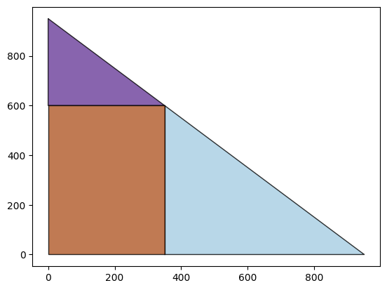
Plot the solution#
gana defaults to PPOPT’s plotting function for multiparametric programs
p.draw()
Evaluate the Solution#
The solution can be evaluated for different values of thetas
p.eval(100, 400), p.eval(200, 300)
({x[0]: 100.0, x[1]: 0.0, x[2]: 0.0, x[3]: 400.0},
 {x[0]: 200.0, x[1]: 0.0, x[2]: 0.0, x[3]: 300.0})
The evaluations get saved in evaluation (dict) and can be accessed
p.x[0].evaluation
{0: {(100, 400): 100.0, (200, 300): 200.0}}
The full solution#
Can be accessed in Program.solution (dict)
p.solution
Solution(program=<ppopt.mplp_program.MPLP_Program object at 0x000002BF571A34D0>, critical_regions=[Critical region with active set [0, 2, 3, 5]
The Omega Constraint indices are [1]
The Lagrange multipliers Constraint indices are []
The Regular Constraint indices are [[0, 2, 3], [1, 6, 7]]
  x(θ) = Aθ + b
 λ(θ) = Cθ + d
  Eθ <= f
 A = [[ 4.55111174e-16 -9.58101146e-17]
 [-1.08095644e-16  2.63420819e-16]
 [ 1.00000000e+00  2.71726164e-17]
 [-4.43739537e-16  1.00000000e+00]]
 b = [[ 3.50000000e+02]
 [ 3.02929788e-14]
 [-3.50000000e+02]
 [ 1.05252933e-13]]
 C = [[0. 0.]
 [0. 0.]
 [0. 0.]
 [0. 0.]]
 d = [[ 12.72792206]
 [323.89350102]
 [261.53967194]
 [ 45.        ]]
 E = [[ 7.07106781e-01  7.07106781e-01]
 [-1.00000000e+00 -2.71726164e-17]
 [ 4.43739537e-16 -1.00000000e+00]
 [ 0.00000000e+00 -1.00000000e+00]]
 f = [[ 6.71751442e+02]
 [-3.50000000e+02]
 [ 1.05252933e-13]
 [ 0.00000000e+00]], Critical region with active set [1, 2, 3, 6]
The Omega Constraint indices are [0]
The Lagrange multipliers Constraint indices are []
The Regular Constraint indices are [[0, 1, 2], [0, 4, 5]]
  x(θ) = Aθ + b
 λ(θ) = Cθ + d
  Eθ <= f
 A = [[ 1.00000000e+00  2.09065079e-16]
 [ 1.08808090e-16  1.00000000e+00]
 [-2.11921834e-16  2.07793336e-17]
 [-2.85118428e-17 -1.47477738e-16]]
 b = [[ 8.57310942e-14]
 [-6.00000000e+02]
 [-8.21908157e-14]
 [ 6.00000000e+02]]
 C = [[0. 0.]
 [0. 0.]
 [0. 0.]
 [0. 0.]]
 d = [[ 50.91168825]
 [308.30504375]
 [323.89350102]
 [ 45.        ]]
 E = [[ 7.07106781e-01  7.07106781e-01]
 [-1.00000000e+00 -2.09065079e-16]
 [-1.08808090e-16 -1.00000000e+00]
 [-1.00000000e+00  0.00000000e+00]]
 f = [[ 6.71751442e+02]
 [ 8.57310942e-14]
 [-6.00000000e+02]
 [ 0.00000000e+00]], Critical region with active set [2, 3, 5, 6]
The Omega Constraint indices are [0, 1]
The Lagrange multipliers Constraint indices are []
The Regular Constraint indices are [[0, 1, 2, 3], [0, 1, 4, 7]]
  x(θ) = Aθ + b
 λ(θ) = Cθ + d
  Eθ <= f
 A = [[1.00000000e+00 0.00000000e+00]
 [0.00000000e+00 1.45579955e-18]
 [6.05443585e-17 0.00000000e+00]
 [0.00000000e+00 1.00000000e+00]]
 b = [[0.]
 [0.]
 [0.]
 [0.]]
 C = [[0. 0.]
 [0. 0.]
 [0. 0.]
 [0. 0.]]
 d = [[308.30504375]
 [261.53967194]
 [ 36.        ]
 [  9.        ]]
 E = [[ 1.00000000e+00  1.45579955e-18]
 [ 6.05443585e-17  1.00000000e+00]
 [-1.00000000e+00  0.00000000e+00]
 [ 0.00000000e+00 -1.00000000e+00]]
 f = [[350.]
 [600.]
 [  0.]
 [  0.]]])
p.A
[[1, 1, 0, 0], [0, 0, 1, 1], [-1.0, 0, -1, 0], [0, -1.0, 0, -1]]
p.P
[[0, 1], [2, 3], [0, 2], [1, 3]]
p.G
[[1, 1, 0, 0], [0, 0, 1, 1], [-1.0, 0, -1, 0], [0, -1.0, 0, -1]]